A Mexican Convenience Store Mexican Standoff
There are two major competitors in the Convenience Store industry in Monterrey, Mexico: “OXXO”” and “7 Eleven”. People usually don’t realize how big is the footprint they have in the metropolitan area. Taking advantage of inegiRand leafletR packages I decided to do a quick visual exercise to learn who is where
About the inegiR package
A couple of months ago I read about inegiR- a R package that helps you interact with the APIs from the official statistics agency of Mexico INEGI within R. Its author @eflores89 talks about the package in r-bloggers in more detail.
It’s important to note that you can access all the information through two APIs - so you are going to need two different tokens. One will give you access to the Indexes while the other one will allow you to pull data from the DENUE database (National Statistic Business Directory… or something like that)
You can get your tokens through these links:
Warming up with the Indexes API
Okay, assuming you already got your tokens, the next step will be to jump into R and load the library…
library(inegiR)… and load the tokens. It’s not that I don’t like to share, but you would have to input your own tokens to make this work.
token <- "abc"
token_denue <- "123"
Once you have the library up and running, and your tokens values stored in some variable then we can start pulling data from INEGI. There are many data sets you can obtain, but for testing purposes I am going to download the Mexican Peso vs USD Exchange rate for the past 20 or 30 years.
cambio <- series_tipocambio(token)
names(cambio) <- c("Cambio", "Fechas")
head(cambio, 5)
## Cambio Fechas
## 1 0.4810 1986-02-01
## 2 0.4831 1986-03-01
## 3 0.5063 1986-04-01
## 4 0.5404 1986-05-01
## 5 0.6312 1986-06-01Now that the data is loaded we can get “fancy”” and load it into some htmlwidget package. Using the dygraphs package we can make a time-series chart.
library(dygraphs)
library(xts)
library(data.table)
r <- xts(cambio, order.by=cambio$Fechas)
dygraph(r, main = "Tipo de Cambio (MXN vs USD)") %>%
  dyRangeSelector(dateWindow = c("1995-01-01", "2015-12-01"))
What about the other API?
To obtain information from the National Statistic Business Directory database (or whatever the exact translation is) we need to use the DENUE API. We already loaded the token a couple of lines above, and now we are going to start using it to download the Convenience Store data.
The formula we are going to use (denue_inegi) requires a specific point and the radius (in meters) that you want to search. The radius has a limit of 5Km and that could be a problem, but later we are going to talk on ways to bypass it. For this exercise we are going to pick the Lat/Lon for the ITESM University and we are going to pull any business that is classified as “comercio al por menor”
latitud = 25.650443 #Tec de Monterrey Campus Monterrey Latitud
longitud = -100.289725 #Tec de Monterrey Campus Monterrey Longitud
mapa <- denue_inegi(latitud,longitud, token_denue, metros = 5000, keyword = "comercio al por menor")
Once we have the raw business data, we’re going to filter to get only stores that have “OXXO”, “ELEVEN” or “EXTRA” in their formal or informal names (Nombre, Razon).
data_etl <- function(mapa=mapa){
oxxo <- mapa[mapa$Nombre %like% "OXXO" | mapa$Razon %like% "OXXO",]
seven <- mapa[mapa$Nombre %like% "ELEVEN" | mapa$Razon %like% "ELEVEN",]
extra <- mapa[mapa$Nombre %like% "EXTRA" | mapa$Razon %like% "EXTRA",]
oxxo$type <- "OXXO"
seven$type <- "SEVEN"
extra$type <- "EXTRA"
output <- rbind(oxxo,seven,extra)
return(output)
}
a <- nrow(mapa)
mapa <- data_etl(mapa)
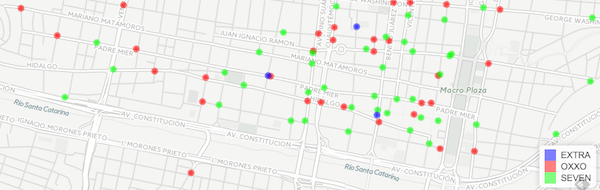
b <- nrow(mapa)Now we have reduced our data frame from 9049 down to 360. Using the leafet package we can now see where are all the stores located 5000 mts around the ITESM.
Working around the radius limit
As we mentioned before, the API only allows to pull data from up to 5Km around your initial coordinates. In order to cover the whole metropolitan area we would need to pick lat/lon points around and loop the points in the denue_inegi formula.
This is a Packing Problem but for now, we don’t want to take it too serious.
This is why I created a function grid that split any rectangular area in points separated by 0.7 degrees in each direction. According to some guys in the internet $1º=~100Kms$. So by trial and error 0.07º will do the work.
The function overlaps the coverage area creating duplicate values. This is why we use the unique function - within grid- to remove duplication.
grid <- function(lat1=25.827886, lon1=-100.499367, lat2=25.617245, lon2=-100.113159){
  lat = 0.07
  lon = 0.07
  grid_output <- cbind(lat1,lon1)
  x <- abs(round((lat1-lat2)/lat, digits = 0))+1
  y <- abs(round((lon1-lon2)/lon, digits = 0))+1
  for (i in 1:x){
    for (j in 1:y){
      la <- lat1-((i*lat)-lat)
      lo <- lon1+((j*lon)-lon)
      prev <- cbind(la,lo)
      grid_output <- rbind(grid_output, prev)
    }
  }
  return(grid_output)
}

a <- as.data.frame(grid())
Here is a look of all the points we’ll loop the denue_inegi function to cover Monterrey and all other close by cities.
By looping denue_inegi through our self-defined grid function we can now see the whole footprint of the major players in the Convenience Store Industry in the Monterrey Metropolitan Area.
I think this is a good time to wrap this up, but the are many potential uses of this script. You could group the data by postal code to understand any variance, or pair that grouping with income or average age in the region to understand the market.
Now, if you have access to POS data it will be a total different ballgame.
Until next time…
UPDATE
You can find the script to replicate this post here
Subscribe
Subscribe to this blog via RSS.
Categories
R 2
Plotly 1
Knime 1
Leaflet 1
Inegir 1
Retail 2
Español 2
Recent Posts
-
 Posted on 29 Jun 2016
-
Posted on 29 Jun 2016
-
 Posted on 31 Jan 2016
-
 Posted on 25 Jan 2016
Popular Tags
Rtodolist (3) R (2) Web scraping (1) Plotly (1) Knime (1) Machine learning (1) Random forest (1) Leaflet (1) Inegir (1) Retail (2) Español (2)